在使用Excel樞紐分析時，常常為需要加入其他表單的資料一起分析，這時候就需要建立各個表格之間的關聯，這個動作可以在分析時減少來回對照的時間，往後在拉表格的時候也可以那多重分析，讓資料變得更完整。

註1：以下資料為模擬練習用，無任何實質意義

註2：此方法僅適用Excel 2013版以後的，較舊版的可能要花時間找一下關聯在哪裡

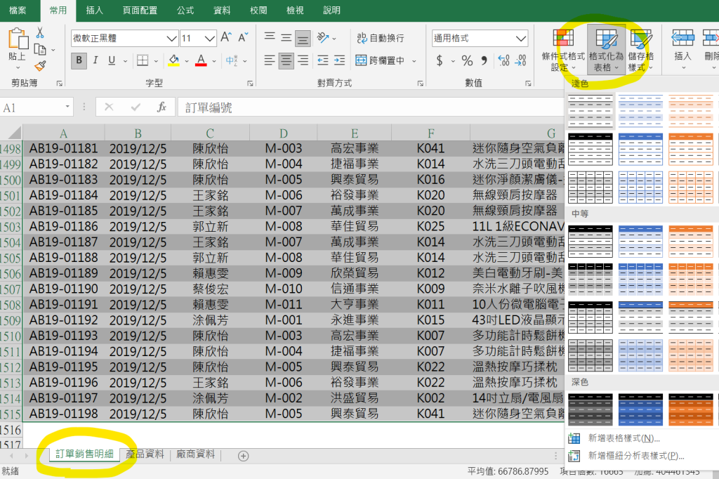
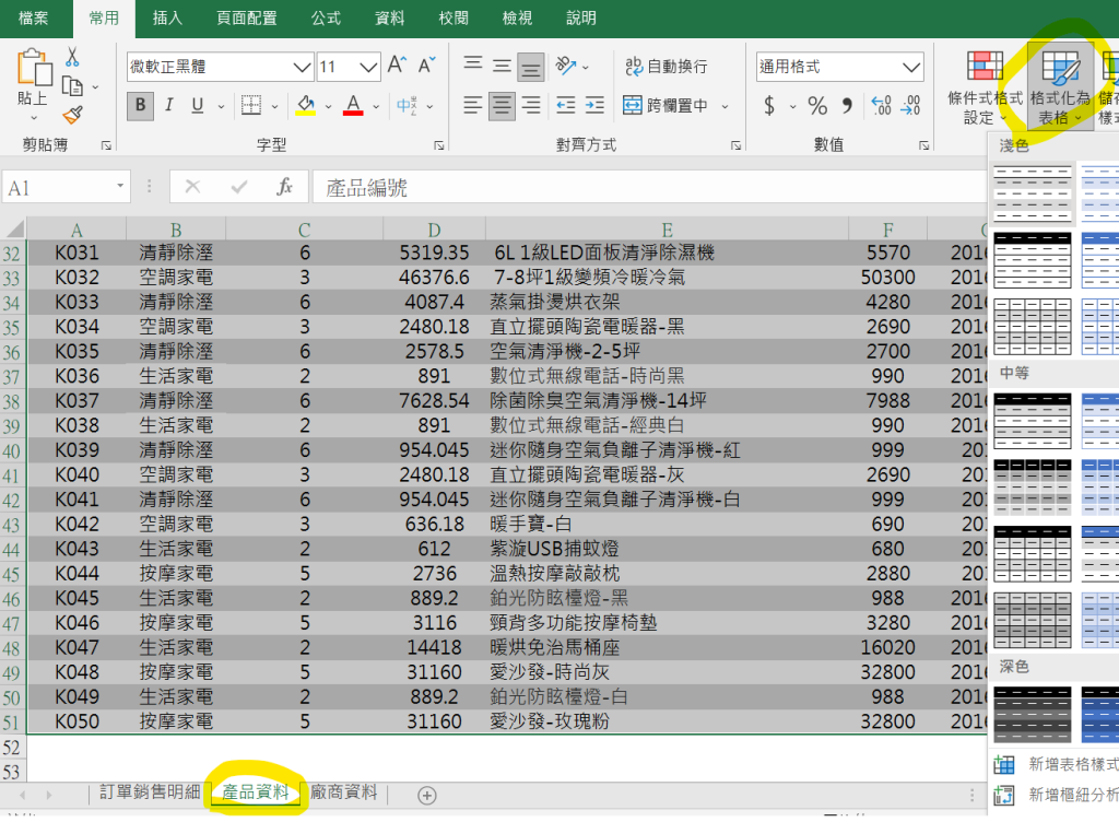
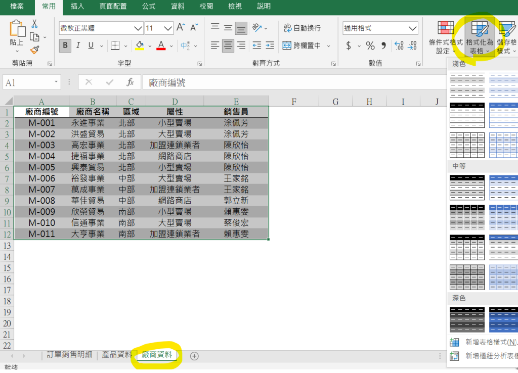
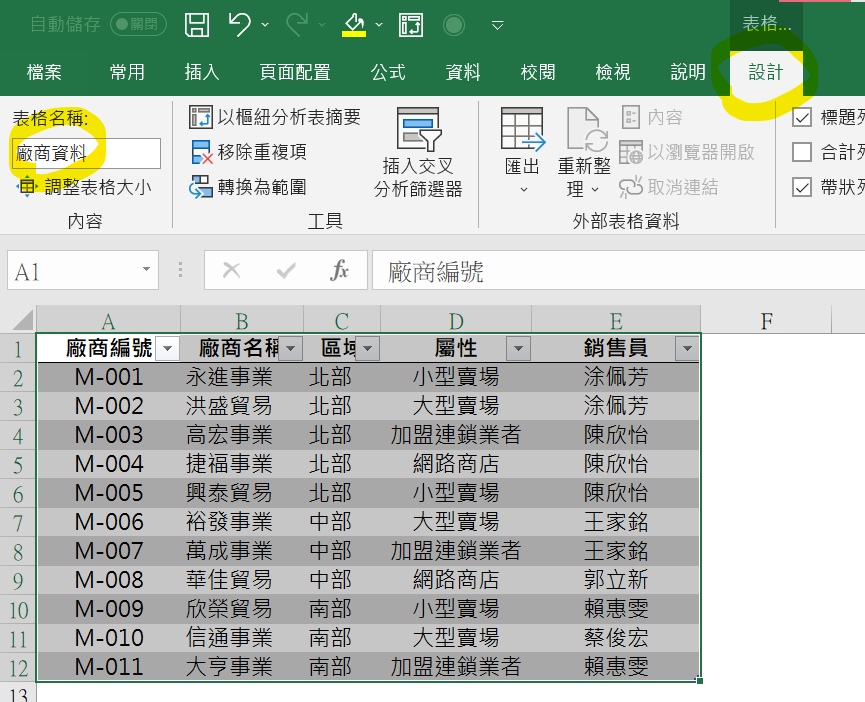
1. 選取欲分析範圍，並點選 “格式化為表格” 將資料換成表格形式

2. 更改表格名稱

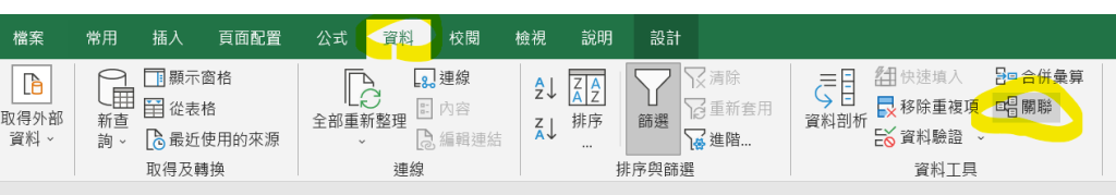
3. 點選 資料> 關聯

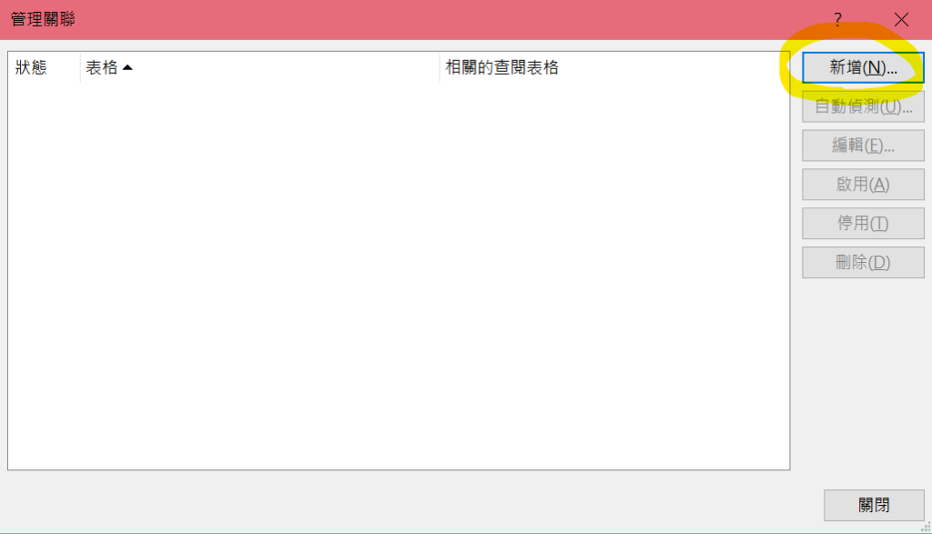
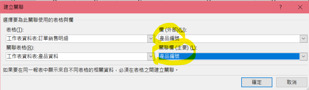
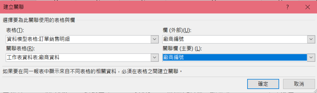
4. 新增表格之間的關聯，建立完成後按關閉

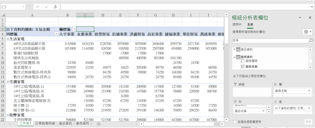
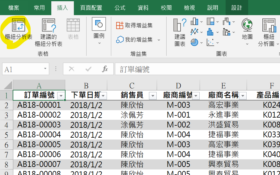
5. 插入樞紐分析表

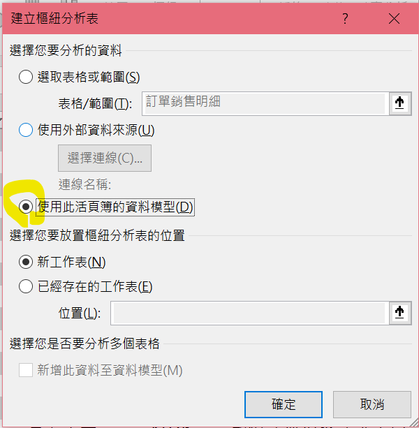
6. 選擇 使用此活頁簿的資料模型

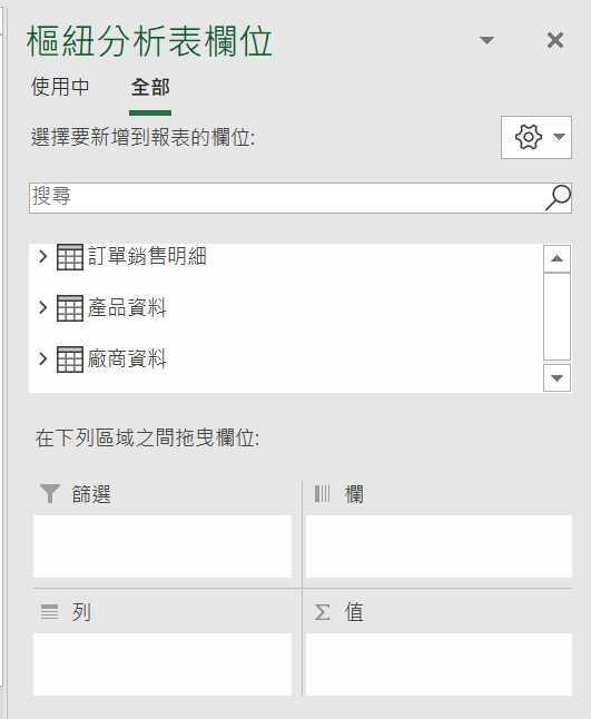
7. 在欄位上就可以看到三個表格內容了！

8. 如此一來就可以跨表格做更全面的分析了！